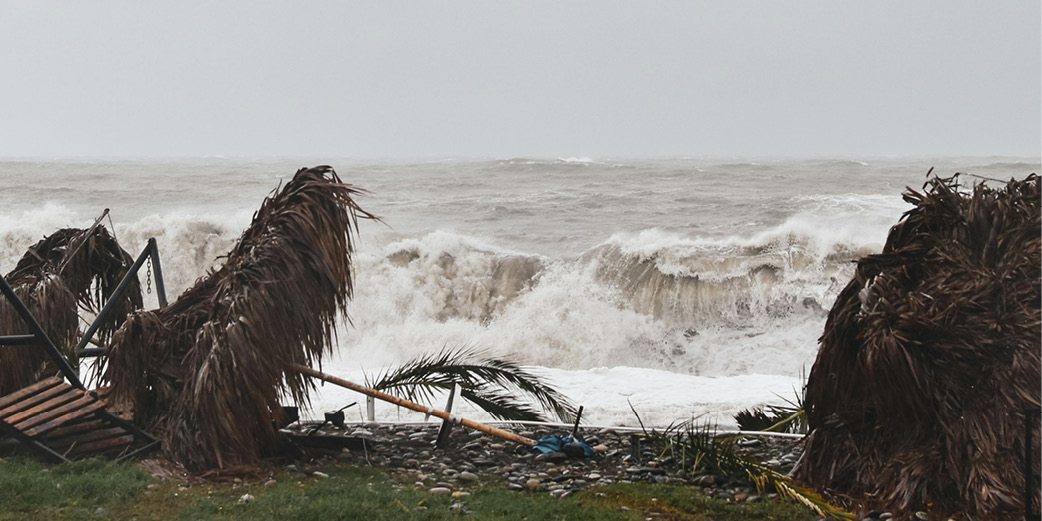
Tropical Cyclone (TC) Alfred hit the central-east coast of Australia on the 8th of March, after generating on the 20th of February and moving south-eastward in the Coral Sea, parallel to the coast. As it moved, it drew heat and moisture from the upper ocean, leaving an imprint in the surface of the ocean and in the waters below.
We were curious to see how TC Alfred’s imprint in the ocean shows up in the figures of the website. Our figures show changes in sea level, surface waves, sea surface temperature, and temperature and salinity in the top 50 meters of the ocean.
Sea level
The easiest way to spot TC Alfred in our maps is by looking at the adjusted sea level anomaly (SLA) map off northeast Australia (Fig 1), which includes atmospheric isobars. In Figure 1, the colours show adjusted SLA values, and the cyan lines are the atmospheric pressure at sea level, spaced at 2 hPa. You can see the closed contours isobars (lines of same atmospheric pressure) forming a coherent feature centred at 153.5°E, 13.5°S on the 23 Feb, that then moves southward over the following week (click forward on the maps, from 23 Feb).
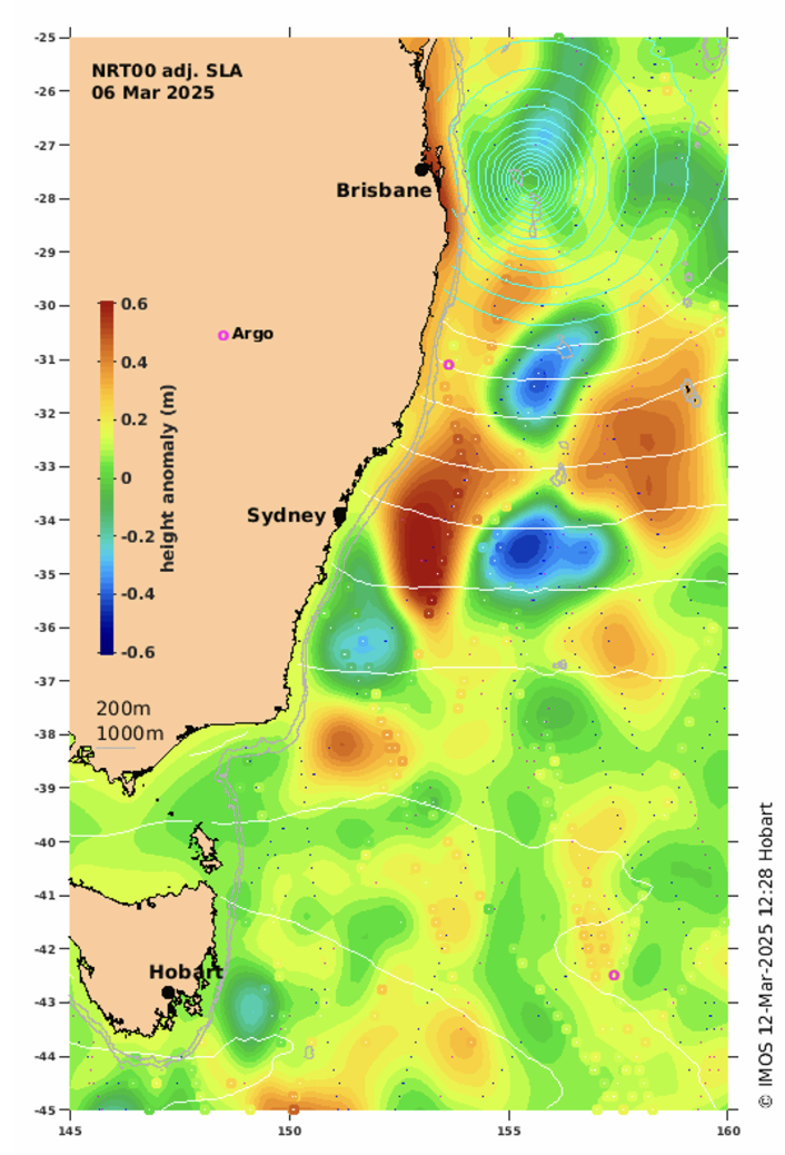
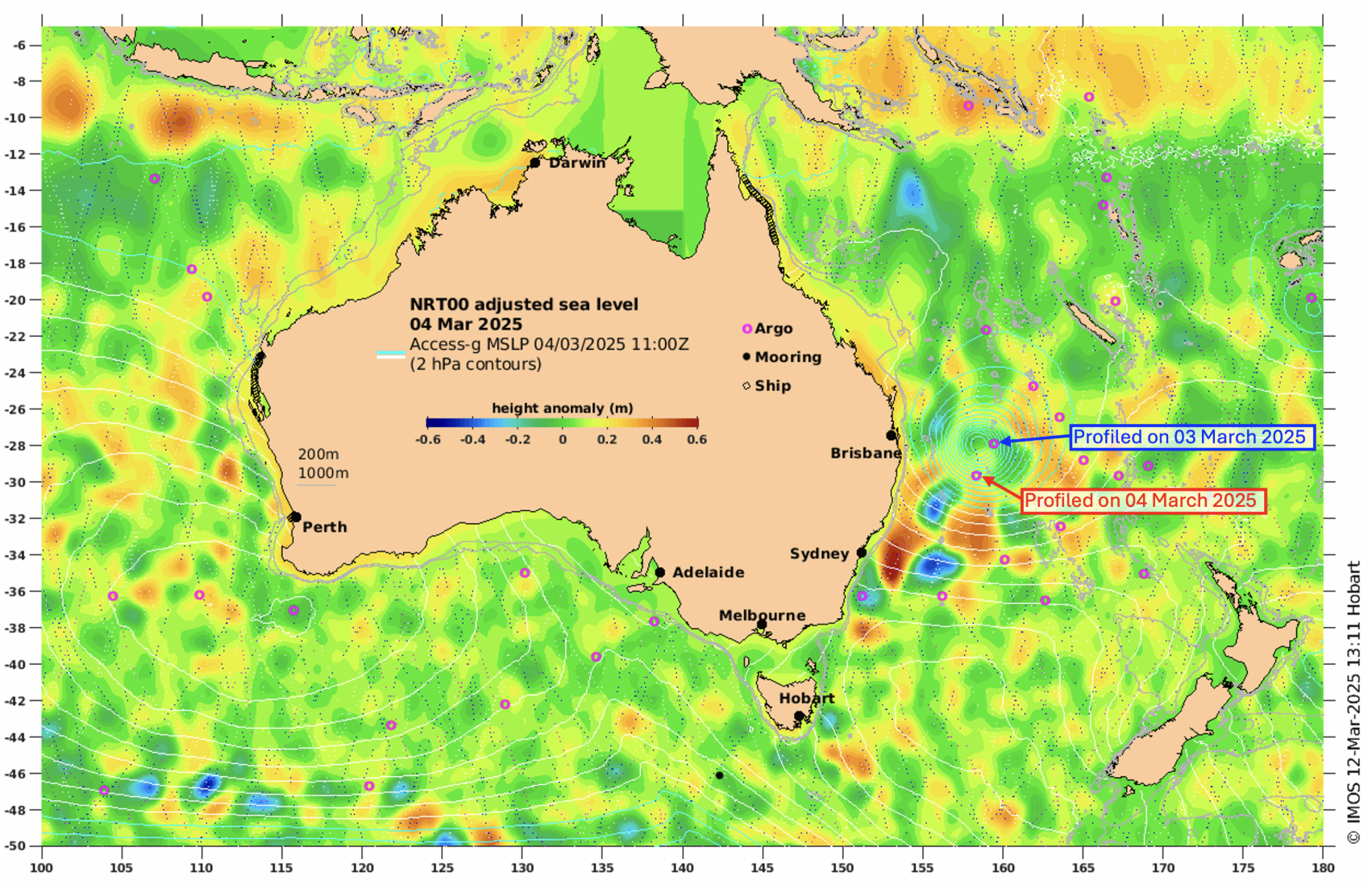
Zooming out to the map of Australia, we see different SLA values immediately below TC Alfred when comparing the maps of adjusted SLA (~ 0 m; Figure 2) and non-tidal SLA (~0.5 m). The values are different because the adjusted SLA has the effect of atmospheric pressure over the ocean removed, while the non-tidal SLA doesn’t. The non-tidal SLA below TC Alfred is high because Alfred has low atmospheric pressure in its centre compared to the surrounding environment. This localised low atmospheric pressure allows the ocean to rise below it.
Surface waves
Cyclones also leave an imprint in the ocean by transferring energy to the ocean through wind friction, forming waves. Surface waves below TC Alfred were over 8 m high, as shown in our surface wave maps from 1st March – read more about TC Alfred and surface waves at the IMOS website.
Sea Surface Temperature
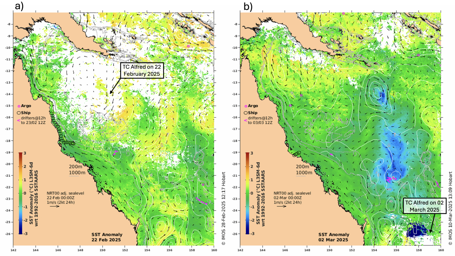
TC Alfred drew heat from the ocean as it moved and intensified, cooling the sea surface temperature on its wake. There was a ~2°C drop in waters of the Coral Sea between 22 February and 2 March (Figure 3). The cooler patch of water after the TC passing is even clearer in maps of SST anomalies.
Note that, on the 2 March, there is a dark blue patch at the southeast corner of the figure, indicating values below the colourbar threshold. These values are non-realistic and are likely caused by difficulties on processing the data near heavy cloud coverage associated with TC Alfred.
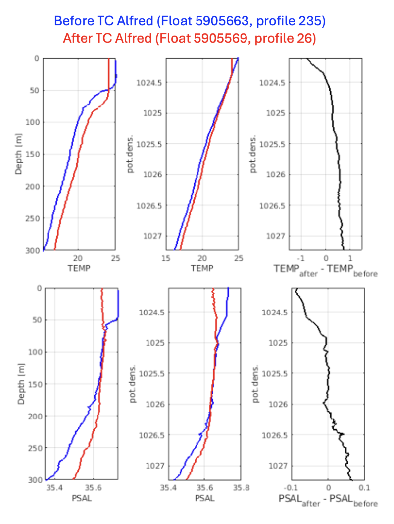
Sub-surface temperature and salinity
An Argo float surfaced right below the cyclone on the 4th of March (red box in Figure 2). We can compare its measurements to the measurements taken by a nearby float at the same location, but before the cyclone passed (blue box in Figure 2).
Figure 4 shows temperature (top) and salinity (bottom) values measured by both floats. The first column shows values plotted against depth (in meters) – showing that the waters at the top 50 meters were warmer and saltier before TC Alfred passed.
The second column shows again temperature and salinity values, but this time plotted against potential density (in kg/m3). This is a better way to compare profiles, because it removes the effect of the vertical movement of the ocean that happened between the days, leaving only the changes caused by mixing and heat exchange.
The third column shows the difference between the temperature and salinity profiles in potential density space – confirming that there was a 0.7°C drop and a 0.1 psu drop in the upper part of the water column after the cyclone has passed.
The freshening seen in the Argo data is a result of heavy rainfall associated with the cyclone, ‘diluting’ the salty waters of the Coral Sea. The cooling is linked to the cyclone drawing heat from the upper ocean, and strong winds mixing the upper layer.
Written by Gabriela S Pilo and David Griffin